Database Internals - How is Time Series data saved?

Introduction
Let’s imagine that we had an idea of a start-up to get the athletes data about their bodies ( heart rates, muscle information, brain signals, breathing, and so on. not only while they are in the matches or training but in almost all day 24 hour. and the startup will be used by the top teams or athletes in the world so they need accurate data in real-time because they will take a decision based on this data for their upcoming events.
Let’s take another example we are using every day. the electric scooters or be-bikes that we can rent for a while. each one of these has a sensor that gives the company the battery status, and location, I do not know the frequency that data will be sent but I think every number of seconds to be aware of it at any time and take actions based on the status of some of them.
You can imagine the size and the high rate of write of such data, how can we deal with something like that from a storage perspective?
As you can see the main point we are talking about here is Time. Everything depends on when the event or data point happened, this type of data can be characterized it as time series data.
Time Series is a series of data points indexed (or listed or graphed ) in time order
This is the definition from Wikipedia. and it is clear enough to describe the time series data. it is any data we care about when it happened and the value at that time.
We are going to talk about how can we save and search through this data.
You will obviously say let’s try one of the available time series databases, and that is not our goal here. Here I will practise with you on how should we think when we are going to think about data storage in cases like time series data. the process of insertion, the algorithm of searching and how can we optimise it
Agreement 🤝
First, we need to agree on how should we consider databases. because for sure we will store such data in a database whatever its type, but the most important thing a database relies on is taking care of how we structure data within the database, It is all about Data Structure here, All these databases rely on effective data structure that give database ability to perform well under high load and it is different based on the nature of data we are aiming to save.
Let's try to think together about how are we going to deal with time series data through different approaches and explain the pros and cons of each approach.
Postgres
We can think about that by applying the electric scooter example here and saving data in the PostgreSQL
| createdAt (Indexed) | id | battery_precentage |
| 2023-05-14T22:36:56.734Z | 1 | 34 |
| 2023-05-14T22:37:56.734Z | 2 | 75 |
| 2023-05-14T22:38:00Z | 3 | 26 |
| 2023-05-14T22:39:00Z | 4 | 78 |
| 2023-05-14T22:40:00Z | 2 | 65 |
Assume we are going to index createdAt column, for better search performance.
Let's see how Postgres handles data insertion, searching, and organizing data ( which data structure) within it.
We need to keep in mind that the time series data nature is heavy writing and searching within a huge volume of data.
Postgres Insertion
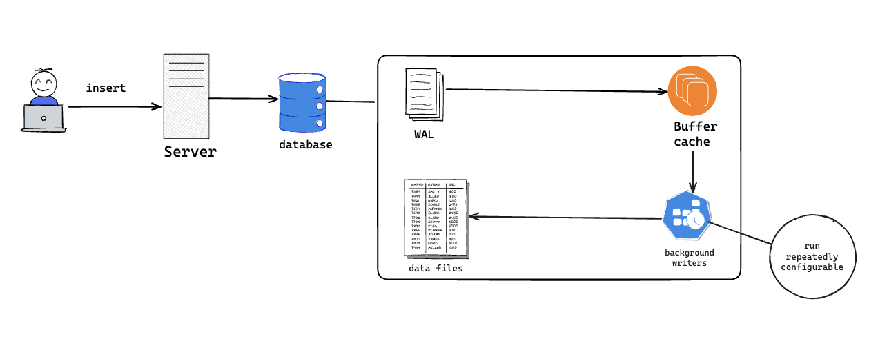
Postgres do the following steps
WAL
What?
WAL is a file that we are only appending to it the operation we are doing in data ( insert, update, delete)
Appending only makes it so fast since we do not care about searching within it
It is more like a journal to save everything that happened to the database
Why?
It is a safe place to keep your operation log in in case of failure.
example: update a record and a server went down for some reason when the database restarts it will do operations that did not complete.
Buffer Cache
What?
- It is space in RAM that Postgres uses for storing the latest returned rows, recently inserted rows, and updated index
Why?
- By doing that we reduce the unnecessary I/O disk workload, by returning the data from the Buffered Cache directly it will be faster and more efficient
Background Writers
There are background writers who work frequently on data that is manipulated in the Buffered Cache to flush it to disk data files. how frequently these background writers will run is configurable e.g.: 30-second
Checkpoint
This happens after background writers flush the data to disk. please pay attention here it is very critical in Postgres, Why? because this is the point that marks in the WAL file that all data in WAL and in Buffered Cache is flushed to disk and all of them are synced now, so if the failure happens and the database restarts the database will read and apply the operation that saved in WAL after last checkpoint
This very abstract overview of insertion in Postgres. But you need to understand this to assist Postgres with time series data.
So far things are going well and fast, We are pushing data to disk not immediately but in batches which makes it efficient, but we are not only flushing data to disk we have an index we need to maintain 🤔
Postgres Indexing
Here we need to remember the very important point we mentioned earlier which is data structure, how we organize our data or an index to search within our data. and that is simply what any index in a database or even a book is doing making access to what you need quickly using the shortest path to it.
There are different types of indexes in Postgres let's assume here we are going to use B-Tree or B+Tree
Introduction to BTree and B+Tree Index
Since we mentioned that the index will give you the opportunity to take the shortest path to access what you want, B-Tree as the name describes is a tree and Postgres saves the index data in a way that helps you to take the shortest path to get your data pointer in disk
BTree
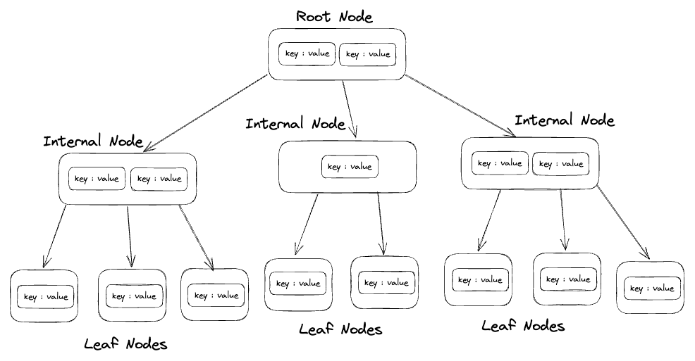
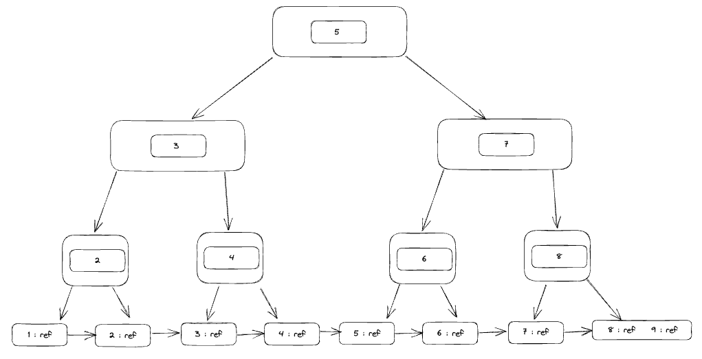
As you can see in the diagram above a Btree is a tree consisting of a root node internal nodes and leaf nodes Each node contains elements The number of elements in the node is determined by the number of children based on this equation m-1 since m is the number of children of this node, as you can see here
Root Node: contains three children so there are 2 elements in the node since
3-1=2Internal Nodes: The middle one has 1 element inside it because it has 2 children
Leaf Nodes: It is the last node so there are no children of course
Also node in the BTree is a page ( page in Postgres is 8kb) so the node will contain a longer amount of elements This example is just a demonstration
this m is called the degree so it could be 3, 4, or 5, In the real world Postgres allows you to adjust this using the following property fillfactor For example, if you want to create an index and specify the degree or order you can do the following
CREATE INDEX idx_example ON your_table(column_name) WITH (fillfactor = 70);
The default value of Postgres is 90, and the range is 10-100 but the smaller you set the degree the more space this index will take in the disk
Inside each element is a key and value
key: is the physical value of the identifier (PK)
value: represents the place reference of this value
So what happened in the query or insertion?
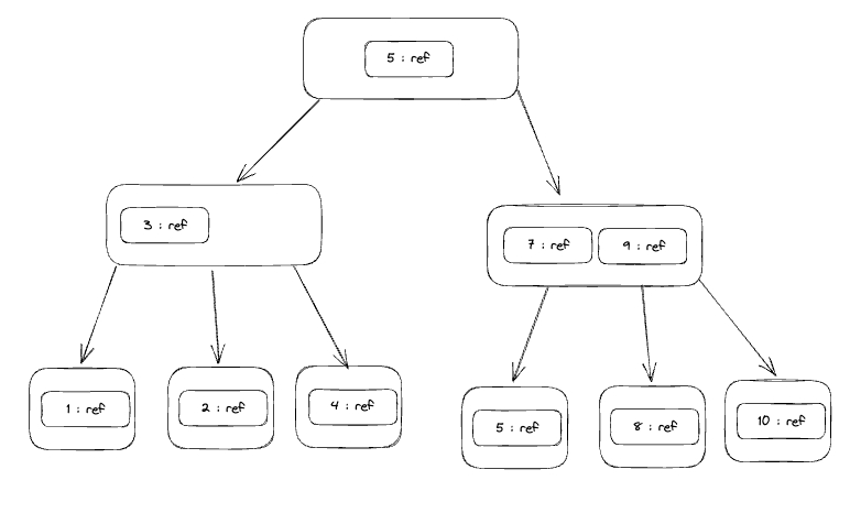
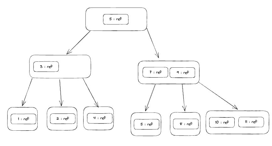
Let's say we have such a BTree index for a PG table this how the index will be look like if we visualize it, what about if I need to insert a new element?
it will look like this, it will search where to add this to the index by checking the root node to decide which direction 11 > 5 then take right Then we have 7 and 9 in the next node so it will be bigger than 9 so we will put it after 10 but we have this tree with degree 3 so each internal node can only have three children so we are going to the node that contains 10 Be ready to be an internal node by adding 11 to it and so on.
what about querying? For example, we need to get the row with ID 8
So we are going to start from the root (disk read) and then go to the right (another disk read) Is it here No we need deeper but it is between 7 and 9 so we go to the middle one and return it so we did a 2 disk reads and loaded them in memory to check them and for later usage if someone needs it.
So the BTree index is somehow not that efficient because :
the elements save key and value and maybe we have the key large like saving uuid so you can imagine the performance
second we can not do the range search, we are trying to save time series data and the range query will be the most popular one, To get such we will do a lot of I/O operations to get all the data that fits this range
The last part B+Tree will solve for us Let's see how.
B+Tree
As you can see first B+Tree eliminates the ref in the elements but still, we have the same concept of degrees. it will save only the key until we reach the leaves, the leaves will contain the references.
This will help us more in query ranges which was a huge downside in the BTree index Also it saves the space of the index in the disk since we are not saving the ref in the internal nodes but only in leaves if there is a sequential query needs to scan the table it will be easier since the leaves are connected.
Now we understand how the insertion and the query are done in the Postgres let's map this to our case of saving and querying time series data.
We have an agreement on the nature of time series data which is heavy write and query ranges so let's check the following
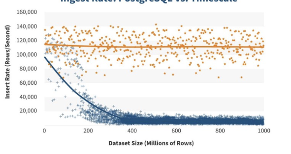
Insertion: Can you imagine with each insert which happens a lot we are going to update the index tree and balance it with the new value This will slow the insertion in the long way when our index grows this is not good. you can see the insertion rate in the blue one
Query: What about having in the case of electric scooters, the battery percentage in the query like getting the count of scooters within a certain time range with battery percentage group by time using minutes, can you imagine such a query in a huge table with a huge index, because big indices do not improve the performance it makes it worse.
Schema Flexibility: The schema of the table is not that flexible to add new columns and query based on them.
So we need something more flexible that can handle heavy writing and can perform complex queries with aggregations.
Let's check another option which is LSM.
LSM ( Log Structure Merge Tree )
LSM is a data structure used in a lot of high-throughput databases because it is scalable to handle such cases.
So how LSM will help to handle high throughput data?
LSM achieves this using these four components
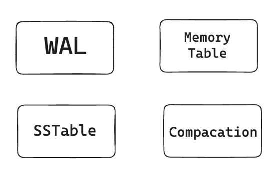
WAL
Memory Table
MemoryTable or memtable is a sorted balanced tree that exists in RAM. MemTable role is to save the incoming data into this sorted tree and once it reaches a certain time it flushes this data "Sorted" to the disk, which makes our disk do nothing regarding sorting the data and caring about what it is sorting. and if there is a failure happened to the machine and memory is cleared, we can load the data from wal and the memtable will sort the data in memory before flushing it to the disk.
SSTable
SSTable stands for "Sorted String Table." It is a file format used in various distributed databases, most notably in Apache Cassandra and Google's LevelDB. SSTables are an important component in these systems for efficient data storage and retrieval.
Compaction
Compaction is a crucial process that helps manage and optimize storage space, improve read performance, and ensure efficient data retrieval.
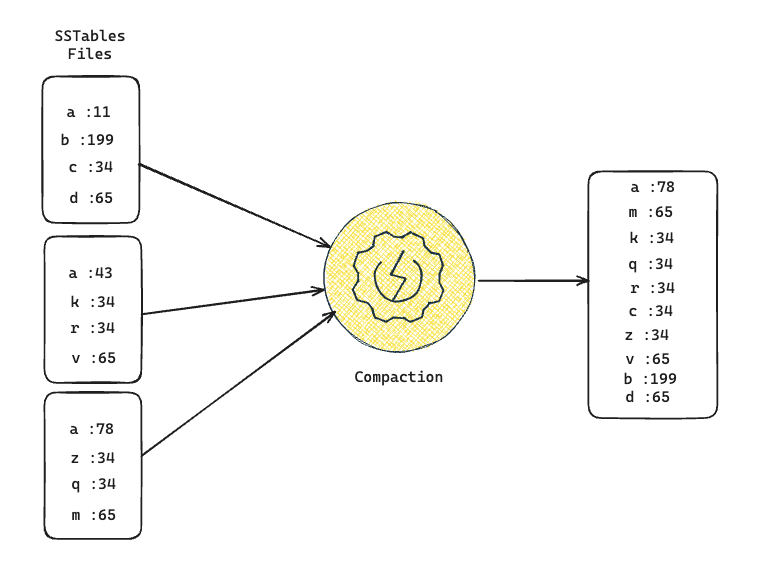
When the number of SSTables in a given level reaches a certain threshold, or when the size of SSTables becomes too large, a compaction is triggered.
During compaction, the LSM tree identifies overlapping SSTables and merges them together into a new SSTable.
Compaction also provides an opportunity to clean up obsolete or deleted data.
Deleted or updated values can be removed, and newer versions of data can replace older versions.
Writing
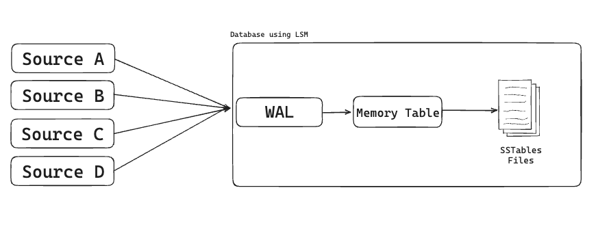
So what happened here is the data came from different resources and reached the server so the WAL write these operations for later and send it to the memory table (memtable) which is a sorted balanced tree on RAM that will take these value and sort them
Once the size of the tree reached a certain size these data were flushed to SSTable files which are immutable files and the data is already sorted so no need to do extra logic on it
Reading
So now you need to query these data, first once your query reaches LSM check first the memtable if the data exists on it to get it which is faster than scanning the disk.
If it is not in the memtable then LSM will scan the SSTables files sorted from newest to oldest. but scanning the disk will make the search not that efficient, then what?
There are multiple ways to overcome this issue
Sparse Index
It works as follows, it takes the key at the start of each SSTable file
  SSTable-0: ["aaabc":0, "aabc":980, "bbcd":1500]
  SSTable-1: ["bcd":2000, "ccc";2200, "ccd":2500]
  SSTable-2: ["cde":3000]
so the sparse index will be like this, has each key at the beginning of the SStable file and its offset so we can reach it easily.
  "aaabc" : 0
  "bcd" : 1000 // offset
  "cde" : 2000 // offset
Advantage
for sure Sparse index will help us to reduce the search space, if we have a full index of all keys its position will be very huge
Less memory space, with fewer keys in the index, requires less memory and storage.
A smaller index means faster looking up
Tradeoffs
- However, there is a trade-off because sparse indexes can introduce additional computational overhead when looking up keys not explicitly listed in the index. The system may need to perform interpolation or other techniques to estimate the position of the key.
Bloom Filter
A Bloom filter is a probabilistic data structure used to test whether an element is a member of a set. It can quickly tell you if an element is "probably" in a set, or "definitely not in the set", but it can have false positives (indicating an element is in the set when it's not) and no false negatives.
Combining both the Bloom filter and Sparse Index will boost our search.
Before accessing the Sparse Index or going to disk, you can first query the Bloom filter to see if the key "may possibly" exist in the dataset.
If the Bloom filter says "no", then you can be reasonably sure that the key doesn't exist. If the Bloom filter indicates that the key may exist, you can then consult the Sparse Index to get a more precise location or estimate of where the key might be within the dataset. This narrows down the search space.
Delete
Deletion in Memory Component (Memtable)
- When a deletion operation is requested, it is first recorded in the in-memory component, often called the "memtable". This involves creating a special entry that indicates the key has been marked for deletion.
Compaction Process
- The deletion marker in the memtable is eventually flushed to disk as part of a regular compaction process. The compaction process is responsible for merging or compacting the data from multiple levels in the LSM tree to ensure efficiency and minimize the number of files on disk.
InfluxDB
![]()
At the beginning let’s give you an introduction to influxDb, InfluxDb is an open-source time-series database designed for efficiently storing, querying, and analyzing time-series data. Time-series data consists of data points associated with timestamps, making it ideal for tracking changes over time. InfluxDB is well-suited for a wide range of applications, including monitoring, sensor data, financial data, IoT (Internet of Things) applications, and more.
so for sure, you are asking what is the difference or the upgrade that InfluxDB gives to us. The best way to learn something is by walking through an example to understand how it works.
For example, let’s imagine we have a hotel with rooms and each room has a sensor that sends data about the room’s weather and we need to save it in influxdb.
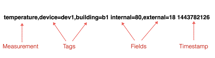
So these rooms send us data and we need to save it in influxdb how or where? we are going to create a measurement to save these data, What is the measurement?
Measurement
It is a logical container that groups similar data points with the same data schema. measurement is more like a table if we think about it as a table in a relational database
examples of measurements are weather measurement, CPU measurement
For example, we need to save the temperature and humidity of each room in the hotel and the sensors send this data each 5 seconds. and each room is marked by its number + floor number like room 1 on floor 1 and room 1 on floor 2 and so on.
How measurement will save these attributes?
Temperature and Humidity influxdb treats them as fields (key and value)
Room number and Floor number influxdb treats them as tag (key and value)
So for example, we are going to save a temperature with a value of 36 and a humidity value of 22 for room number 3 on floor 1. In influxdb will be like that
weather,room=3,floor=1 temprature=33 humidity=22
so we are going to save this value like a row in a table like any relational database, right? Hmm actually no there is something called Series in influxdb, Wait again what? What is the series?
A series represents a specific collection of data points that share the same measurement, tag set, and timestamp
It is the fundamental unit of data in InfluxDB. Each data point belongs to a series, and the series is identified by its SeriesKey, which is formed by the measurement name and tag set
Series belongs to measurement, so measurement could have multiple series
if we need to apply this definition to our example. We are going to have a series per room and floor
Series 1:
Measurement: "weather"
Tags: "floor" = "1", "room" = "1"
Fields: "temperature" = 25.0, "humidity" = 50.0
Unique Series Key: "weather,floor=1,room=1"
Series 2:
Measurement: "weather"
Tags: : "floor" = "1", "room" = "2"
Fields: "temperature" = 22.5, "humidity" = 60.0
Unique Series Key: "weather,floor=1,room=2"
Series 3:
Measurement: "weather"
Tags: : "floor" = "2", "room" = "3"
Fields: "temperature" = 23.8, "humidity" = 55.5
Unique Series Key: "weather,floor=2, room=3"
and so on ...
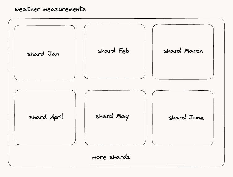
Okay, I got it but this series will grow exponentially, how does influxdb manage this?
Actually, influxdb is dividing data in shards each share represents a range of time-series data points. Shards are often associated with specific time ranges, such as a day or a week.
Let's do what we did in the previous options
How does influxdb perform insertion and querying? But first's let's understand some concepts
InfluxDB Concepts
It is the same as LSM but with slightly couple of differences
WAL
The WAL here is doing the same as others but it is used to keep the fresh added data until it reaches a certain time or a certain size, both of them are configurable, then it flushes the data into the TSM files on the disk and it will not be removed from the WAL until it receives confirm that the data successfully flushed to the disk.
While this flushing operation happening if the newly added data fills within the query's given time range it will be returned with the results that give more power for the querying
The WAL keeps an in-memory cache of all data points that are written to it. The points are organized by the key, which is the measurement, tagset, and unique field. Each field is kept in its own time-ordered range. The data isn’t compressed while in memory.
Deletes sent to the WAL will clear out the cache for the given key, persist in the WAL file, and tell the index to keep a tombstone in memory.
And for sure these WAL files are backed up to use later in a failure or damaged case
Cache
Like any other database influxdb depends on cache (RAM) to optimize the query time and make reach to the frequently accessed data to be retrieved faster. How is influxdb using cache to achieve that?
Influxdb uses the memory (RAM) to save the location of the data points, not the actual data points, Why? this makes sense since the amount of data is quite huge in one query You can imagine how many data points are retrieved which will exceed the memory and make it inefficient. so Influxdb saves this cached data points' location in the cache and calls it the TSM Index (In-Memory Index). The TSM Index is a data structure that resides in memory and contains information about where data is stored on disk. It helps InfluxDB quickly locate and retrieve the relevant data during queries. saving the location of accessing this data will allow for faster lookups. This reduces the need to access disk storage for index information, which can be a relatively slow operation since we know in the end that we save the actual data index on disk.
How is the cache kept updated?
Write Operations:
When new data points are written to the database, the TSM Index is updated to include information about the location of the newly written data on disk.
This ensures that subsequent queries can quickly locate and retrieve the relevant data
Compaction:
InfluxDB periodically performs a process called compaction. Compaction combines smaller TSM files into larger ones to optimize storage and improve read performance.
During compaction, the TSM Index is also updated to reflect the new structure of the merged files.
Cache Eviction:
- In some cases, if the available memory for the cache is limited, InfluxDB may need to evict less frequently accessed data from the cache to make room for more recently accessed data.
Background Maintenance:
- InfluxDB performs various background tasks to ensure the integrity and performance of the data and indices. These tasks may include things like disk cleanup, metadata updates, and index optimizations.
TSM (Time-Structured Merge Tree)
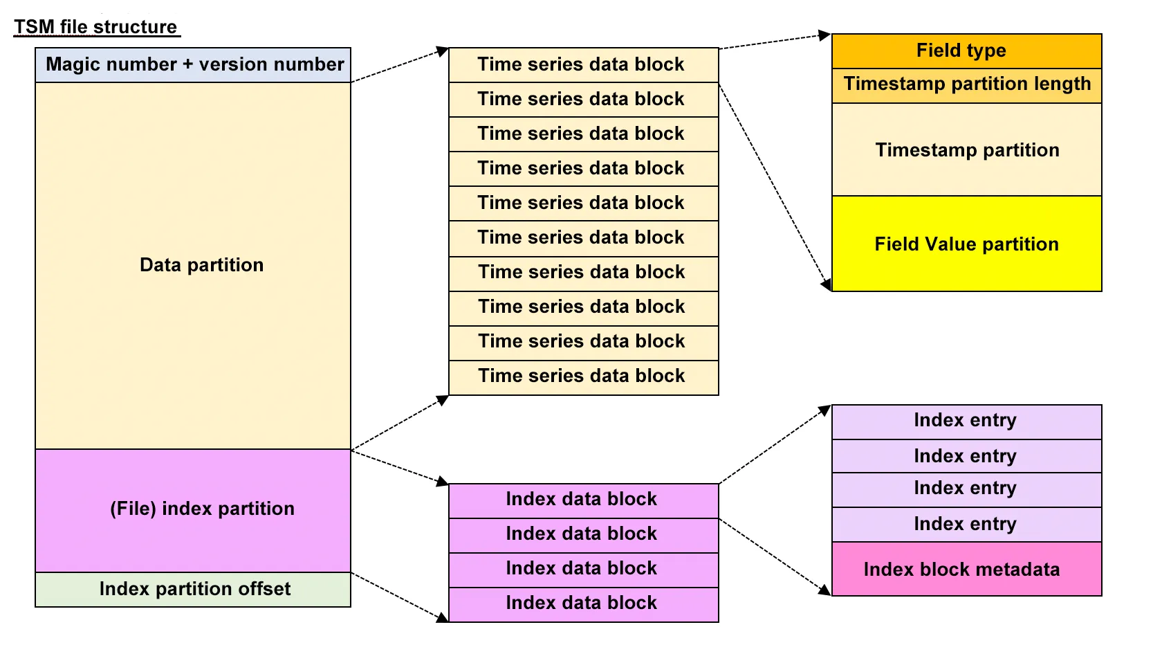
TSM file consists of the following
Header: consists of magic number as id and version number
Data Partition: this consists of data blocks each data block contains data points for different series not only one series
Block Index
consist of
block Id: data block Id
start time
end time
offset in the TSM file
Block Entries
a block entry refers to a single data point within a data block.
consisting of
timestamp
field value
series key ID ( the ones saved in the names file)
field key ID ( the ones saved in the names file)
Series Key Index
- Here we are saving the series key which exits in this TSM file, this helps influxdb a lot to get the data from TSM files more fast and efficiently
Field Key Index
TSI (Time Structure Index)
Influxdb saves the index that helps us access the data in something called TSI. TSI uses an on-disk index structure that is optimized for time-series data. It organizes data in a way that allows for efficient range scans and point lookups. The TSI index is based on a B+ Tree data structure. This structure is well-suited for efficient range queries, which are common in time-series data.
Also, Influxdb is having compaction for the TSI as well. but combining the small index files into larger ones will optimize the disk space and search space.
Long story short it is the same B+Tree and instead of PK values in the root and internal nodes we have here the hashed key (hashed series kery) and the leaves as you know it is the reference of this key location.
Writing
Once a new data point reaches influxdb, for sure it writes it on the WAL until the time to flush it to disk (TSM file)
Influxdb creates a unique ID of series key (measurement + tag) per tag and another one for field keys for each data point, takes these values, and feeds each one into a hash function for example (fnv-64) which produces a unique ID for each one then save them in a file called "names", these will be used while reading to filter the data points exist in the TSM files
Sometimes hash function produces the same ID for multiple keys, so influxdb creates a collision file that saves all these IDs to resolve them while reading as we are going to see in the next section.
influxdb consults the index to see where it will save the new data point by knowing which shared and the place of this data point in the TSM file.
Reading
so now there is a query that asks to get data from the first floor from last week? how can this be translated to influxdb to do the search?
since we have a huge volume of data the key thing here is to reduce the scanning of irrelevant data.
Then we have a time range ( last week ) so we will pass the from and to dates with the query which will help influxdb to do a binary search within the segments we have that are divided based on time ranges.
By that, we eliminate the segments we will check ✅
Then influxdb will take the series key ( measurement + tag set) we passed ( in the current example is weather [measurement] and floor one [tag] ). and pass this key to the hash function influxdb has to get the key of this series key(ID), to get the locations of this series key in the TSM files that exist in the segment we have will happen in different places but first we need to check collision
check the collision file
collision file is the file in which we save the series keys that have the same hash value, this should not always happen but this is a fallback for the hash function if the same hash key for different series keys.
The collision file maps hash values to hash buckets, each containing a list of series keys that have hashed to the same value.
For each hash bucket in the collision file, additional data is stored to differentiate between the series keys.
influxdb checks the file by searching by generated hashed key and each key has a bucket of the series keys that correspond to it with additional data to differentiate these series keys
Then start searching for the locations in TSM files within:
check the TSI ( Time Series Index)
TSI is proposed in the new influxdb engine, it is an index that is based on B+Tree.
The B+Tree indexing is used to map series keys (measurement names and tag sets) to their corresponding locations within the TSM files.
check the index cache
- influxdb always checks the cache for series keys that may be recently used, these series keys always have their locations. for sure that reduces Disk I/O and optimizes the search
Once we get the date we decompress the data points save them into the cache for later usage and return the results to the user
Delete
Deletes are handled in two phases. First, when the WAL gets a delete it will persist it in the log, clear its cache of that series, and tell the index to keep an in-memory tombstone of the delete. When a query comes into the index, it will check it against any of the in-memory tombstones and act accordingly.
Later, when the WAL flushes to the index, it will include the delete and any data points that came into the series after the delete. The index will handle the delete first by rewriting any data files that contain that series to remove them. Then it will persist any new data (for this series or any others), remove the tombstone from memory and return success to the WAL.
Update
Updates are held first in the WAL. If there are a number of updates to the same range, ideally the WAL will buffer them together before it gets flushed to the index. The index will rewrite the data file that contains the updated data. If the updates are to a recent block of time, the updates will be relatively inexpensive.
And if you want to update the field and timestamp, it is not recommended you should delete the point and insert a new one.
Conclusion
In this part, we explored different types of databases to solve time series data use cases, explored if we used PostgreSQL how it handles such data volume in all read and write, also saved what is the next thing we can start with to take a step further for better performance in read and write using LSM but more depending on memory (RAM) storage sorted data and flushed it to disk, then we discussed more improved/ enhanced version which is influxdb that used both the LSM methodology somehow (depending on RAM memory before flush data to disk without sorting) and using B-tree index and how it deals with write and read.
I hope you enjoyed this explanation and added something for you, and see you more in the next database internal exploring articles.
Thank you :)
